DaSPi — Process Analytics & Six Sigma in Python

DaSPi helps engineers analyze and improve processes using statistical workflows.

🎯 The Problem

Process analysis in practice is fragmented:

• Excel is error-prone and hard to scale
• Minitab / JMP are expensive and closed
• Python tools (pandas, scipy, statsmodels) are powerful but disconnected

👉 Engineers spend more time combining tools than improving processes.

✅ The Solution

DaSPi provides integrated workflows for process analytics:

• Capability analysis (Cp, Cpk)
• Root cause analysis (ANOVA, regression)
• Statistical process control (SPC)
• Professional visualization

All in one consistent and intuitive interface.

🚀 Four Flagship Workflows

DaSPi provides four ready-to-use workflows that cover the complete quality cycle. Each workflow produces visual output + interpretation in under 20 lines of code.

---

📏 Workflow 1: Gage R&R Analysis

Verify your measurement system is capable before analyzing process data.

import daspi as dsp

# Load data
df = dsp.load_dataset("grnr_layer_thickness")

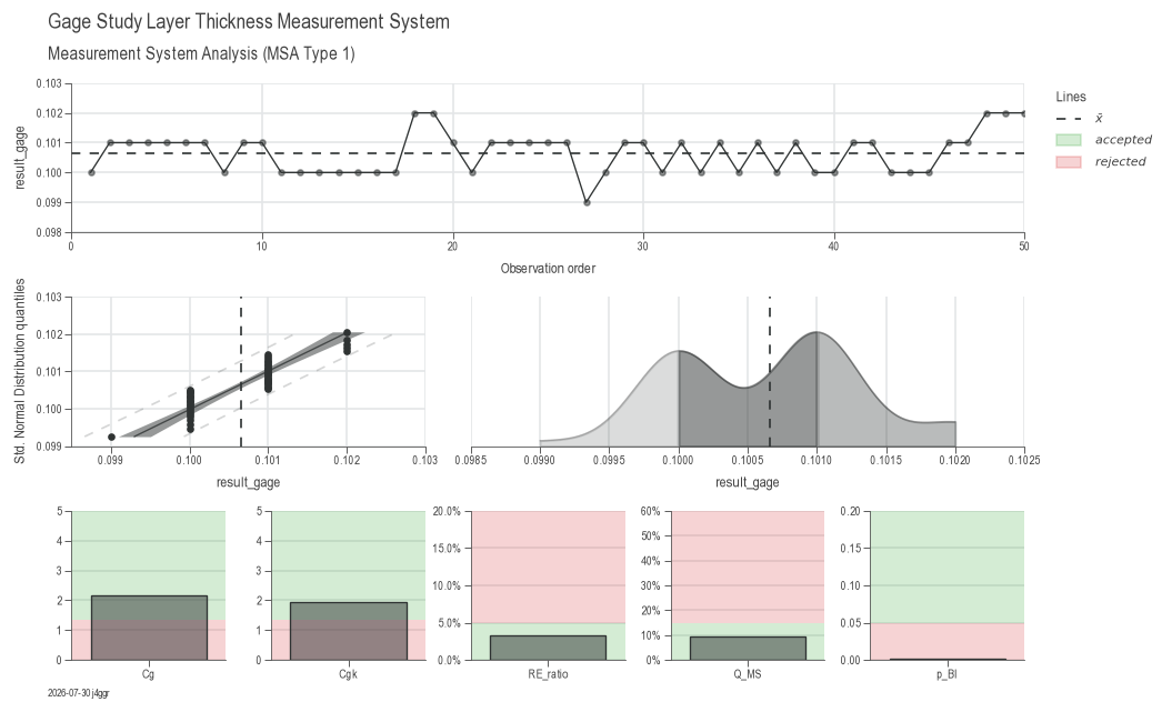
# Step 1: Evaluate the gage itself (MSA Type 1)
gage = dsp.GageStudyModel(
    source=df,
    target="result_gage",
    reference="reference",
    u_cal=df["U_cal"][0],
    tolerance=df["tolerance"][0],
    resolution=df["resolution"][0]
)

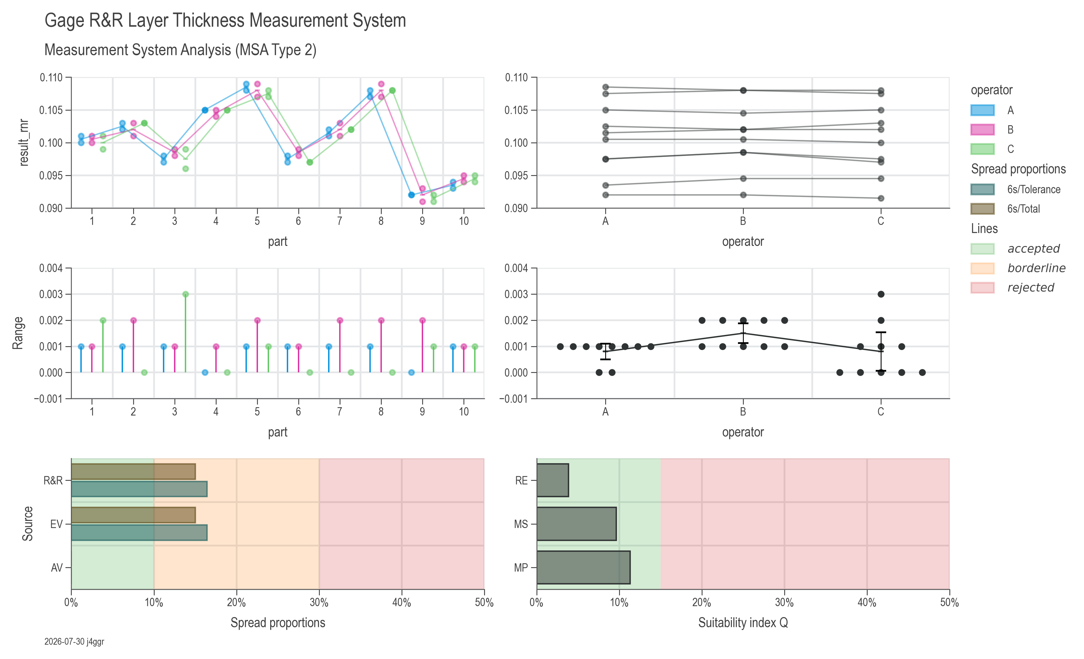
# Step 2: Evaluate repeatability & reproducibility (MSA Type 2)
model = dsp.GageRnRModel(
    source=df,
    target="result_rnr",
    part="part",
    gage=gage,
    u_av="operator"  # Operator variation
)

# Step 3: Visualize complete analysis
chart_gage = dsp.GageStudyCharts(
        gage,
        stretch_figsize=1.5
    ).plot(
    ).stripes(
    ).label(
        fig_title='Gage Study Layer Thickness Measurement System',
        sub_title='Measurement System Analysis (MSA Type 1)',
        info=True)

chart_rnr = dsp.GageRnRCharts(
        model,
        spread_accepted_limit=0.1,   # 10% threshold for acceptance
        spread_rejected_limit=0.3,   # 30% threshold for rejection
        u_accepted_limit=0.15,       # 15% uncertainty threshold
        stretch_figsize=1.5
    ).plot(
    ).stripes(  # Adds acceptance zones
    ).label(
        fig_title='Gage R&R Layer Thickness Measurement System',
        sub_title='Measurement System Analysis (MSA Type 2)',
        info=True)

Output: Comprehensive measurement system evaluation with repeatability (EV), reproducibility (AV), variance components, ANOVA tables, and capability indices (Cg, Cgk).

---

📊 Workflow 2: Process Capability Analysis

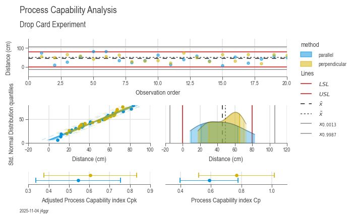
Evaluate if your process meets specifications.

import daspi as dsp

# Load data
df = dsp.load_dataset("drop_card")
spec_limits = dsp.SpecLimits(0, float(df.loc[0, "usl"]))

# Analyze capability
chart = dsp.ProcessCapabilityAnalysisCharts(
    source=df,
    target="distance",
    spec_limits=spec_limits,
    hue="method"
).plot().stripes().label(
    fig_title="Process Capability Analysis of Drop Card Data",
    sub_title="Drop Card Distance Comparison between Two Methods",
    target_label="Distance s (cm)",
    info=True)

chart.show()

Output: 5-panel analysis with Cp, Cpk, Pp, Ppk, distribution plots, and statistical interpretation.

---

🔍 Workflow 3: Root Cause Analysis

Identify which factors significantly impact your process.

import daspi as dsp

# Load data
df = dsp.load_dataset("painkillers-dissolution")

# Fit model with automatic factor selection
model = dsp.LinearModel(
    source=df,
    target="dissolution",
    factors=["employee", "brand", "water", "catalyst"],
    covariates=["temperature"],
    order=2,
)

# Perform recursive elimination to select significant factors
df_gof = pd.concat(model.recursive_elimination())

# Visualize results
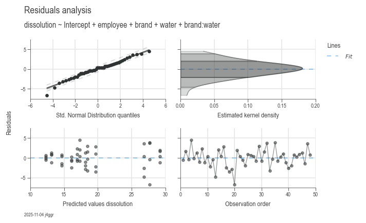
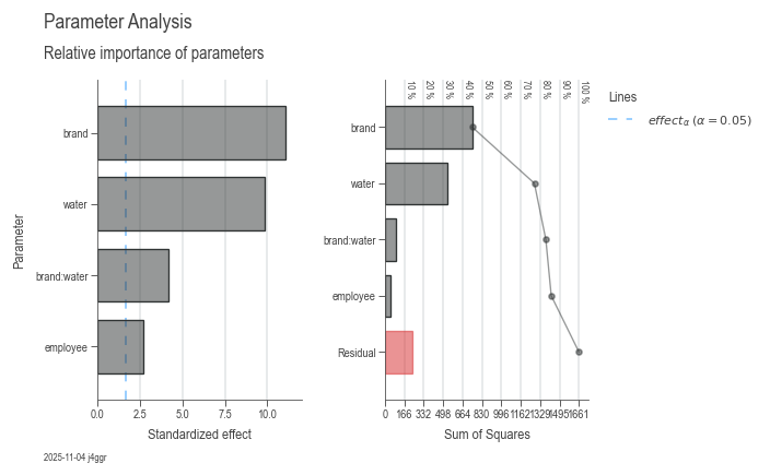
chart_res = dsp.ResidualsCharts(model).plot().stripes().label(info=True)
chart_param = dsp.ParameterRelevanceCharts(model).plot().stripes().label(info=True)

Output: Residual diagnostics + parameter effects with ANOVA tables and significance tests.

---

📈 Workflow 4: Statistical Process Control (SPC)

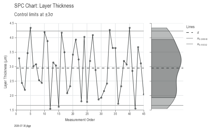
Monitor process stability and detect out-of-control conditions.

import daspi as dsp

# Load process data
df = dsp.load_dataset("grnr_spc")

# Create control chart
chart = dsp.JointChart(
        source=df,
        target='result',
        feature=('measurement_order', ''),
        nrows=1,
        ncols=2,
        width_ratios=[4, 1],
        sharey=True,
    ).plot(
        dsp.Scatter
    ).plot(
        dsp.Line,
        on_last_axes=True,
    ).plot(
        dsp.GaussianKDE,
        hide_axis='feature',
        visible_spines='target',
    ).stripes(
        mean=True,
        control_limits=True,    # UCL/LCL at 3-sigma
        agreement=3,            # 3-sigma agreement lines
        strategy='norm',        # Use normal distribution for control limits
    ).label(
        fig_title='SPC Chart: Layer Thickness',
        sub_title='Control limits at ±3σ',
        target_label='Layer Thickness (µm)',
        feature_label=('Measurement Order', ''),
        info=True
    )

chart.show()

Output: Control chart with mean, control limits (UCL/LCL), specification limits, and trend analysis.

🏭 Use Cases

• Manufacturing: Monitor tolerances and reduce defects
• Quality Engineering: Automate Six Sigma DMAIC workflows
• Process Optimization: Identify key drivers of variation
• Data Analysts: Unify statistics and visualization in one tool

📊 Example Outputs

MSA1: Gage Study (Single Reference)

MSA2: Gage R&R (Repeatability & Reproducibility)

Process Capability Analysis

Root Cause Analysis (ANOVA)

formula:

dissolution ~ 26.8292 + 2.3750employee[T.B] + 0.8375employee[T.C] - 10.7500brand[T.ZapPain] - 9.5167water[T.tap] + 5.7167*brand[T.ZapPain]:water[T.tap]

Model Summary:

	hierarchical	least_parameter	p_least	s	aic	r2	r2_adj	r2_pred
0	True	employee	0.023298	2.374693	224.835935	0.857379	0.840400	0.813719

Parameter statistics:

	coef	std err	t	p	ci_low	ci_upp
Intercept	26.829167	0.839581	31.955433	0.000000	25.134824	28.523509
employee[T.B]	2.375000	0.839581	2.828793	0.007133	0.680657	4.069343
employee[T.C]	0.837500	0.839581	0.997522	0.324224	-0.856843	2.531843
brand[T.ZapPain]	-10.750000	0.969464	-11.088598	0.000000	-12.706458	-8.793542
water[T.tap]	-9.516667	0.969464	-9.816417	0.000000	-11.473125	-7.560208
brand[T.ZapPain]:water[T.tap]	5.716667	1.371030	4.169616	0.000149	2.949817	8.483516

Analysis of variance:

Typ-I	DF	SS	MS	F	p	n2
employee	2	46.431667	23.215833	4.116891	0.023298	0.027960
brand	1	747.340833	747.340833	132.526821	0.000000	0.450027
water	1	532.000833	532.000833	94.340328	0.000000	0.320355
brand:water	1	98.040833	98.040833	17.385695	0.000149	0.059037
Residual	42	236.845000	5.639167	nan	nan	0.142621

Variance inflation factor:

	DF	VIF	GVIF	Threshold	Collinear	Method
Intercept	1	5.000000	2.236068	2.236068	True	R_squared
employee	2	1.000000	1.000000	1.495349	False	generalized
brand	1	1.000000	1.000000	2.236068	False	R_squared
water	1	1.000000	1.000000	2.236068	False	R_squared
brand:water	1	1.000000	1.000000	2.236068	False	single_order-2_term

SPC: Control Chart with Mean, UCL/LCL, Specification Limits

🚀 Installation

pip install daspi

📚 Documentation

• User Guide — Complete tutorials for each workflow
• API Reference — Detailed documentation
• 3S Methodology — Structured problem-solving

🔧 Technical Features

• Centralized configuration — Manage language, username, and styles globally
• Multivariate visualization — Explore complex relationships
• Linear models & ANOVA — Statistical inference made simple
• Hypothesis testing — Confidence intervals and p-values
• Monte Carlo simulation — Assess uncertainty
• Process capability — Cp, Cpk, Pp, Ppk calculations

⚙️ Built on Proven Libraries

DaSPi leverages the Python scientific stack:

• pandas — Data manipulation
• numpy — Numerical computing
• matplotlib — Visualization
• scipy — Statistical functions
• statsmodels — Advanced statistics

👤 About

DaSPi is created and maintained by Reto Jäggli, Data Scientist at Festo Microtechnology AG.

The project is driven by a passion to make process analytics and Six Sigma workflows more accessible in Python.

⚠️ Disclaimer

DaSPi is under active development and may contain bugs.
Results should be validated with trusted statistical tools when required.

🤝 Feedback & Contributions

If you use DaSPi in real-world process analysis:
👉 I would love to hear your use case.

Feedback, ideas, and contributions are very welcome.

---